I believe that a solid foundation in numerical methods is crucial for accurately representing complex physical phenomena in computational models.
In the context of fluid mechanics, my academic and professional journey has equipped me with a deep understanding of numerical methods applied to the Navier-Stokes equations. I am well-versed in discretization techniques, including finite volume method, which are essential for solving partial differential equations governing fluid flow. These methods enable the transformation of continuous mathematical models into discrete approximations, allowing for the numerical solution of complex fluid dynamics problems
Furthermore, I have experience with Reynolds-averaged Navier-Stokes (RANS) methods, particularly in turbulent conditions. My familiarity with the discretization of turbulent terms and the application of appropriate boundary conditions is essential for achieving accurate and stable simulations.
In addition to my academic background, my programming skills further support my application of numerical methods. I have successfully implemented these methods in various programming languages, including MATLAB, Processing, Phyton… This versatility allows me to adapt to different computational environments and apply numerical methods effectively in the context modeling.
finite volume and finite element methods
Finite Volume Method (FVM) and Finite Element Method (FEM) are numerical techniques used for solving partial differential equations (PDEs) in the context of fluid dynamics and other engineering applications.
Finite Volume Method (FVM):
Concept:
- FVM discretizes a physical domain into small control volumes (or cells).
- The governing equations are integrated over each control volume to obtain discrete algebraic equations.
- It conservatively represents the integral form of the governing equations.
Equation Setup:
- In fluid dynamics, the conservation laws (e.g., mass, momentum, energy) are often represented by partial differential equations.
- FVM discretizes these equations by evaluating the fluxes at the faces of each control volume and integrating over the volume.
Conservation:
- FVM inherently satisfies conservation principles, making it well-suited for problems involving fluid flow and heat transfer.
Application:
- Commonly used in CFD simulations for fluid flow problems, combustion, and heat transfer.
Finite Element Method (FEM):
Concept:
- FEM divides a physical structure or domain into smaller elements.
- The behavior of each element is described by simple mathematical expressions.
- The overall solution is obtained by assembling the contributions of all elements.
Equation Setup:
- Governing equations are transformed into a weak form, involving spatial and temporal variations.
- Shape functions, representing the behavior of elements, are introduced to interpolate the field variables.
Flexibility:
- FEM is highly flexible in handling complex geometries and material properties.
- It is well-suited for problems with irregular boundaries or heterogeneous materials.
Application:
- Widely used in structural analysis, heat transfer, electromagnetics, and fluid dynamics.
- In fluid dynamics, FEM is often applied to problems with complex geometries and moving boundaries.
- Control Volumes vs. Elements:
- FVM focuses on discretizing the physical space into control volumes.
- FEM divides the domain into elements, each described by a set of simple functions.
- Conservation:
- FVM naturally conserves quantities as it directly discretizes the integral form of conservation laws.
- FEM may require additional care to ensure conservative behavior.
- Geometry Handling:
- FVM is typically easier to apply to simple geometries.
- FEM excels in handling complex geometries and irregular boundaries.
Both methods have their strengths and weaknesses, and the choice between them often depends on the specific characteristics of the problem at hand.
one-dimensional steady-state momentum equation for an incompressible fluid
Let’s consider the one-dimensional steady-state momentum equation for an incompressible fluid. The equation is:

where u is the velocity, μ is the dynamic viscosity, and p is the pressure.
Finite Volume Method (FVM):
Discretization:
- Divide the domain into control volumes.
- The equation is integrated over each control volume.
Integration:
- Apply the divergence theorem to convert the spatial derivatives into surface integrals.

Flux Calculation:
- Express the flux terms using the values at the faces of the control volumes.

Spatial Discretization:
- Apply a spatial discretization method to approximate spatial derivatives (e.g., central differencing).

The Reynolds-Averaged Navier-Stokes (RANS) method
Certainly! The Reynolds-Averaged Navier-Stokes (RANS) method is a widely used approach in computational fluid dynamics (CFD) to simulate turbulent flows. Let’s break down the key concepts and steps involved in RANS:
The Navier-Stokes equations describe the motion of fluid, taking into account the effects of viscosity and inertia. However, solving the full unsteady Navier-Stokes equations for turbulent flows is computationally expensive. RANS is an approach that aims to model the effects of turbulence without explicitly resolving all the turbulent scales.
Turbulence is inherently unsteady and chaotic, but RANS assumes that turbulent quantities can be decomposed into mean and fluctuating components. Time-averaging is a fundamental step in RANS, where all quantities are decomposed into mean and fluctuating components:


The time-averaged Navier-Stokes equations can be written as the sum of mean and fluctuating components:
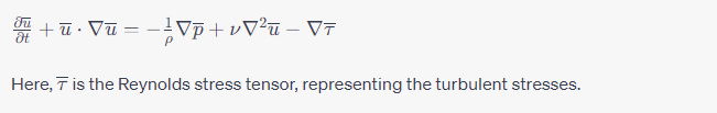
The Reynolds stress tensor involves unknown quantities and requires closure. Closure is achieved through turbulence models, which are mathematical formulations that provide an expression for the Reynolds stress terms based on the mean flow properties.
Common turbulence models include:
- Spalart-Allmaras Model
- k-ε Model (k-epsilon)
- k-ω Model (k-omega)
- Reynolds Stress Model (RSM)
Each model has its advantages and limitations, and the choice depends on the characteristics of the flow being simulated.
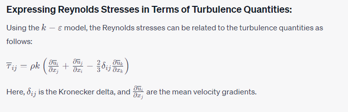
The k-ε model is a popular RANS model. It introduces two additional transport equations for

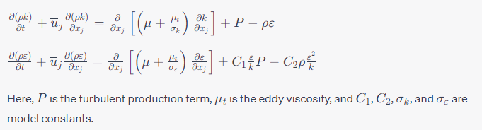
In Reynolds-averaged Navier-Stokes (RANS) simulations, turbulent flows are characterized by additional stresses, known as Reynolds stresses that represent the effects of turbulent fluctuations on the mean flow. These stresses are the key components in the extra terms added to the mean flow equations.
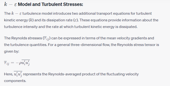

Represents the intensity of turbulence at a point. High values of (k) indicate high turbulence intensity.

Represents the rate at which turbulence is being dissipated. It provides information about the energy transfer from turbulence to heat.
Solution Procedure:
- The additional transport equations for (k) and (E) are solved along with the mean flow equations.
- Using the solved values of (k) and (E), the Reynolds stresses are then calculated and incorporated into the mean flow equations.
Solver Implementation:
The entire set of equations (mean flow equations + (k-E) equations) are then implemented in a numerical solver, often using finite volume or finite element methods. The solver discretizes the domain, solves the equations, and iterates until a converged solution is obtained.
Validation:
The accuracy of the simulation is often validated against experimental data or benchmark cases to ensure that the chosen turbulence model and solver settings are appropriate for the specific flow conditions.
obtaining steady-state solutions by solving time-averaged equations.
Time Averaging:
- RANS assumes that turbulent flows can be decomposed into mean and fluctuating components. The time averaging is performed over a sufficiently large and representative time period.
Steady-State Equations:
- The governing equations (Navier-Stokes equations) are then time-averaged to obtain steady-state equations with additional terms representing turbulence effects. These additional terms involve Reynolds stresses, which are modeled using turbulence models.
Solution for Steady-State:
- The RANS equations are solved numerically to obtain the steady-state mean flow variables, such as mean velocity, pressure, etc.
Statistical Stationarity:
- The time-averaging process assumes statistical stationarity, meaning that statistical properties of the flow do not change significantly over the averaging time.
Turbulence Modeling:
- Turbulence models are crucial in RANS to close the equations by providing expressions for Reynolds stresses. These models account for the effects of turbulence on the mean flow.
Application in Engineering:
- RANS is widely used in engineering simulations to predict the mean behavior of turbulent flows, and it’s computationally more efficient than methods like Large Eddy Simulation (LES) or Direct Numerical Simulation (DNS) for certain applications.
Large Eddy Simulation (LES):
Large Eddy Simulation (LES) is a computational fluid dynamics (CFD) technique used to simulate turbulent flows. In LES, the large energy-containing eddies in the turbulent flow are resolved directly, while the smaller, dissipative eddies are modeled. It’s a compromise between fully resolving all scales of turbulence (as in Direct Numerical Simulation – DNS) and modeling all scales (as in Reynolds-Averaged Navier-Stokes – RANS).
Key Concepts of LES:
- A spatial filter is applied to the governing equations, separating the flow field into resolved (large) and subgrid (small) scales.
- Models are used to represent the effects of the unresolved, small-scale turbulence on the resolved scales. These models capture the interactions between resolved and subgrid scales.
- LES requires a mesh that is fine enough to resolve the large eddies, but not necessarily the smallest ones. The choice of grid resolution is a critical aspect of LES.
- LES is computationally more demanding than RANS but less demanding than DNS. It strikes a balance between capturing important turbulence features and managing computational costs.